
Technological Change and Declining Immigrants’ Earnings Outcomes: Implications for Income Inequality in Canada
Casey Warman and Christopher Worswick

Ce chapitre fait partie de l’ouvrage collectif Income Inequality: The Canadian Story. Il est le fruit de deux années de collaboration entre l’IRPP et le Réseau canadien de chercheurs dans le domaine du marché du travail et des compétences (RCCMTC). Pas moins de 27 éminents experts y analysent les tendances en matière d’inégalité au Canada, les facteurs ayant dicté l’augmentation des inégalités depuis le début des années 1980 et le rôle que doivent jouer les politiques publiques pour remédier au problème.
In 1981, Canada’s only economics textbook on economic inequality concluded confidently that “economic inequality has remained roughly constant since the Second World War” (Osberg 1981, 205). Little did its author then realize how much Canadian inequality, and the study of inequality, was about to change! The 35 years since have seen an explosion of the literature on inequality and remarkable innovations in research methodologies — both of which -undoubtedly have been driven by the changing facts of economic inequality. Nevertheless, although much has been learned in recent years about economic inequality, some important results of the early literature have slipped from view — in particular, the limitations of summary indices of inequality and the futility, in a market economy, of distinguishing inequality of opportunity from inequality of outcome. Meanwhile, the emphasis of the early literature on comparing levels of inequality has unfortunately remained. That emphasis was, in 1980-81, reasonable. When the level of inequality is fairly stable in many countries, as it then had been for several decades, thinking of economic inequality in terms of cross-sectional comparisons of societies makes sense. Such comparisons enabled researchers to ask if countries with higher levels of income inequality are less healthy, less democratic and less happy and have more crime, more conflict and less intergenerational social mobility and equality of economic opportunity than countries with lower levels of inequality. Cross-country comparisons are useful if one can depend on inequality remaining stable and if one is interested in answering a question like “What type of society would one like to live in?” Since this is an important question, and since there was a significant period during which within-country levels of income inequality did not change much, the literature on income inequality has continued to emphasize such comparisons.
However, cross-sectional comparisons between countries presume that observed levels of inequality represent steady-state outcomes (that is, situations that potentially could persist into the indefinite future). But that can be true only when income growth is balanced (that is, if the rate of income growth is equal at all percentiles of the income distribution).1 When income growth is unbalanced, the level of inequality changes over time.
Increasing inequality in a given society, and an expectation that the trend will continue, raise fundamentally different issues from a one-time change in the level of inequality. It is one thing to say that Canada is more unequal now than it was in 1980, and quite another to say that Canada is more unequal now than it was in 1980 and Canadians can expect it to get ever more unequal each year into the indefinite future. In this chapter, therefore, I ask what the implications of ever–increasing inequality might be and whether this can possibly be a steady state.
Specifically, there is no natural upper bound to the real income of those at the top of the income distribution, and thus no natural upper bound to the gap between their income and that of median households. But can an ever–increasing income gap between the top 1 percent and everyone else possibly continue indefinitely? “More inequality,” in the sense of increasing inequality over time, raises important questions: What sort of society are we becoming? What processes could equalize income growth rates across income classes and thereby stabilize the distribution of income? How likely are they to occur? What happens if income growth rates remain unequal?
I begin by asking what can be learned about the long-run implications of higher inequality from comparisons of cross-sectional data. I then compare real income growth rates over time at the very top of the income distribution and for the bottom 90 percent and bottom 99 percent in Canada, the United States and Australia to illustrate how unique the postwar period of balanced growth (and consequent stability of the income distribution) actually was in these three countries. In recent decades, the rapidly rising share of market income of those at the very top end of the distribution has reflected a new normal: unbalanced growth. I then suggest that there is little reason to expect an equalization of market income growth rates any time soon, and I argue that unbalanced growth of incomes cannot be a long-run steady state. Unequal income growth rates imply changes in savings flows that may cumulate to changed stocks of indebtedness, financial fragility and periodic macroeconomic crises. Ever-increasing income gaps also imply increasing top-end spending on political influence and children’s education, as well as ever–increasing incentives to advertise the luxury consumption that fuels envy. Greater macroeconomic, political and social instability is therefore a likely implication of more inequality over time. I conclude by suggesting that, if markets do not spontaneously auto-equilibrate, the political economy of increasing inequality will be crucial, but the outcomes of those processes are very unclear.
By economic inequality, I mean differences among people in their command over economic resources. However, because every society has many different types of economic resources, used by many different people at different points in time, the measurement of inequality depends crucially on being specific about inequality of what among whom, when. Like most of the literature, I focus in this chapter on inequality in the distribution of annual income.2 But to decide which annual income concept is most appropriate to discuss, one first needs to ask why we want to know.
In a market society, income flows perform dual functions. “Market income,” for example, is simultaneously the payments of firms and the receipts of individuals. Firms pay individuals to motivate the supply of labour and capital to the production process, while individuals typically pool their receipts within households to enable personal utility from consumption. If one wants to think about how changes in the size, structure and organization of firms and markets are changing inequality, one therefore should start with inequality among individuals in their receipt of factor payments — that is, their individual market income before tax.
Much of the literature is motivated, however, by concern about inequality in the distribution of well-being from consumption, because equity in well-being is important in a social justice sense. If “inequality” is to be understood in terms of potential consumption, the fact that most people live in households and share consumption with other family members implies that the appropriate annual income concept on which to focus is the total disposable — that is, after taxes and transfers — money income of households. If well-being from the consumption of disposable income is to be measured accurately, some allowance should be made for the economies of scale in consumption that are available to larger households. In affluent countries, therefore, it has become common practice to adjust household income for family size and to report the distribution of equivalent disposable income among all individuals.3 One can thus discuss income inequality either from a production perspective, in terms of the inequality of factor payments (individual market income), or from a consumption perspective, in terms of inequality in household receipts of purchasing power (household market income plus transfers minus taxes). In this chapter, I primarily emphasize the former perspective — that is, trends in the inequality of individuals’ shares of pre-tax market income.
However, an important lesson from the consumption perspective, as Heisz (in this volume, figure 2) illustrates, is that the level of inequality of disposable household income varies considerably among advanced market economies. Although all member countries of the Organisation for Economic Co-operation and Development (OECD) compete in the global marketplace and are -increasingly interconnected in trade and harmonized in market regulation, there is a broad range in levels of within-country inequality of disposable household income. Evidently, the institutional framework of market capitalism and effective participation in the modern global economy do not dictate a unique level of disposable household income inequality; social choices are possible. But since it is hard to imagine that the level of income inequality could be unconnected to other aspects of society,4 an important question then is, “What exactly are the implications of more or less income inequality?”
Over the past 30 years, an ever-expanding group of scholars has used cross-country comparisons to address the implications of inequality. Richard Wilkinson and Kate Pickett’s 2010 book, The Spirit Level: Why Equality Is Better for Everyone, is a particularly famous example. In it, the authors compare the level of inequality of disposable household income with a host of social indicators — average levels of health status, trust, social mobility, infant mortality, educational performance, violence, obesity, mental illness, teenage births, homicides and imprisonment — both across OECD countries and across states within the United States. They conclude that, along all these dimensions, in places where there is more income inequality there are also more social problems.
However, even if more inequality might be guilty of causing these problems, proving it rigorously is difficult. Wilkinson and Pickett use correlations and scatter plots that cannot establish causation, and they depend heavily on data from only 25 affluent countries, which exposes their work to the critique that this or that “outlier” might be dominating their results. As Leigh, Jencks and Smeeding (2009, 399) put it, in discussing the relationship between inequality and health, “a fundamental problem is the fact that this is a field with too many theories for the number of available data points.”
Although many studies (for example, Osberg and Smeeding 2006) have documented that the vast majority of survey respondents in all countries express a preference for less inequality, surveys rarely define the term precisely. Cross-country comparisons indicate, however, that nations differ sometimes in the share of income of those at the top of the income distribution, sometimes in the share of the middle classes and sometimes in the gap between the poor and the rest of society. Which aspect of inequality matters most? In much of the recent academic literature on inequality, there is little evidence of awareness of the complexities of index construction that early literature emphasized.
Like many other recent scholars, Wilkinson and Pickett (2010) use the Gini coefficient as if it were an unambiguous measure of inequality, but Atkinson’s (1970) article on the limitations of using a single number to summarize the many differences in individuals’ access to economic resources remains fundamental. He noted that, among the many possible summary indices of inequality, one should accept only those that satisfy some basic ethical criteria — such as the “principle of transfers” (i.e., that a transfer of income from poor to rich should always imply an increase in any acceptable index of inequality).5 Within the class of such axiomatically defensible inequality indices, the Gini coefficient is more sensitive to income changes in the middle of the distribution than is the Theil index (which is low-end sensitive) or the coefficient of variation (which is high-end sensitive) (see Jenkins 1991; Osberg 1981, chap. 1; Osberg 1984, chap. 1). Atkinson (1970) showed that these indices will agree unambiguously only sometimes in their cross-country rankings of inequality. Specifically, they will all agree that country A has less inequality than country B only when it is always true, at all points in the income distribution, that the relatively poorer in country A have a bigger share of income than comparable people in country B. Atkinson also showed, however, that, in real-world comparisons, it is rare to observe such unambiguous dominance.
To illustrate the ambiguities that can hide beneath simple comparisons of the Gini coefficient, I invented the example of “Adanac,” a mythical country in which the income distribution is very simple: the bottom four-fifths (80 percent) of the population all have the same low income — each quintile group (20 percent) of people gets 10 percent of total income. The income of those in the top 20 percent is exactly six times higher, and thus they get 60 percent of total income (Osberg 1981, 14). In real-world Canada in 2011, the total income share of the poorest 20 percent of the population was actually 4.1 percent, while the share of the richest 20 percent was 47.2 percent. So these assumptions imply that in Adanac, both the extremes of the income distribution would get a substantially bigger share of national income than they do in Canada. However, the middle 60 percent of Adanac, who in total have an income share of 30 percent, are considerably worse off than the middle 60 percent in real-world Canada, whose actual share in 2011 was about 48.7 percent. Which society is more unequal? I picked the numbers for Adanac so that it has approximately the same Gini coefficient as does Canada. But these are very different societies.6 The answer to which is more unequal depends on which part of the income distribution one thinks matters most for inequality: the top-end share, the share of the middle classes or the gap between the poor and everyone else.
Ambiguities of measurement have become particularly relevant for Canada in recent years, since the increase in the Gini coefficient of equivalent household disposable income after 2000 has been much smaller than the increase in the 1990s. However, this flattening of the upward trend in the Gini coefficient masks a trend to the greater polarization of incomes in Canada. Since 2000, the relative advantages of the middle class have declined — that is, the ratio of the average income of the second, third and fourth quintiles to that of the first quintile has fallen. As Beach (in this volume, 171) documents, there has been a “marked decline in the proportion of workers who receive middle-class earnings” in -Canada. Because the incomes of many in the middle class have converged downward toward the incomes of the poor, a perverse sort of equalization of incomes has occurred among the bottom 80 percent. At the same time, the income share of the top 1 percent has continued to increase, but this is obscured in the Gini coefficient, which adds up the absolute value of the income differences among all possible pairs of people. In the calculation of the Gini coefficient, lessened inequality among the bottom 80 percent — that is, the “declining middle class” — is combined with, and offsets, rising inequality at the top end of the income distribution. Most Canadians might think that a declining middle class combined with an increasing share of income for the top 1 percent would amount to more inequality, not the same level of inequality — but that is not how the Gini coefficient is calculated.
Although cross-sectional evidence on many of the social implications of higher levels of income inequality might not be rigorously conclusive, recent literature unambiguously confirms old perceptions about the connection between more inequality of outcome and more inequality of opportunity. As Brunori, Ferreira and Peragine (2013, 7) conclude, using cross-country regressions, “Countries with a higher degree of income inequality are also characterised by greater inequality of opportunity…Less unequal countries are also those that have a higher degree of intergenerational mobility.” Corak (2004, 2013) and many others have made the same point.
The idea that economic inequality accumulates and deepens over generations is hardly new. Indeed, in a market economy in which parents can control their personal expenditures on the human capital of their own children, it is inevitable that the inequality of income of adults will influence the inequality of opportunity of children. As Alfred Marshall (1913, 562) remarked, “The professional classes especially, while generally eager to save some capital for their children are even more on the alert for opportunities of investing it in them” (emphasis in original), while the children of the working classes “go to their graves with undeveloped abilities and faculties.” Marshall insisted especially that “this evil is cumulative,” and generations of sociologists have since confirmed the intergenerational transmission of socio-economic status.
In economics, the best-known neoclassical formalization is the Becker and Tomes (1979) parental altruism model of intergenerational bequest. In this model of human capital acquisition and financial bequest, the unequal distribution of income among cohorts of parents is due partly to their own unequal inheritances from the previous generation, which, in turn, enables unequal transfers to their own children. Inequality in parental income thus has an “income effect” on inequality of opportunity because more parental income enables more disparity in the “enrichment expenditures” (Corak 2013, 91) that increase the skills of advantaged children. Increasing inequality among parents also has a “price effect” in that the widening of the income differential between the “success” and “failure” of their children implies greater incentives for parents to invest private resources in their children’s human capital. In general, the whole notion of equality or inequality of opportunity makes no sense at all in a one-generation model of human behaviour. However, as soon as the human capital model is extended to consider two or more generations, inequality of outcome in one generation inevitably generates inequality of opportunity in the next generation, and a strict distinction between inequality of outcome and inequality of opportunity becomes untenable.
The widespread availability of cross-national data has had the important result of establishing that social choices can be made about the level of income inequality.7 When the level of income inequality could be assumed to be stable, one could use such cross-country evidence to help answer questions such as “What sort of society would one like to live in?” But that was then, and this is now. The level of inequality can remain constant only if incomes throughout the income distribution are growing at the same rate. In Canada, the United States and Australia, this has not been true since the 1980s. Instead, higher rates of income growth at the top end of the distribution are compounding on ever-higher base incomes, and these countries now must ask if this increasing inequality will stabilize, and what the implications are if it does not.
For many years, the United States has had considerably more income inequality than the OECD average, while Australia and Canada have been somewhat closer to, but still above, the mean level of household income inequality in advanced market economies. In all three countries, moreover, the Gini coefficient of inequality in equivalent annual net household income has been trending up, albeit with pauses corresponding to periods of decline in the unemployment rate. In this chapter, however, I focus on the changing real incomes of the top 1 -percent and the bottom 99 percent and 90 percent, for three main reasons.
First, a summary index of inequality does not indicate which parts of the income distribution have changed. In the United States and Canada, there has been remarkably little change in real incomes over the past 30 years for much of the income distribution — the real incomes of the 20th, 40th, median, 60th and 80th percentiles of the family income distribution have been quite flat over time.8
Second, the absolute size of recent changes in the income share of the top 1 percent dwarfs the magnitude of both shifts historically observed and those now occurring elsewhere in the income distribution. Prior to 1980, studying income distribution was sometimes described as being “about as interesting as watching grass grow” (Salverda, Nolan and Smeeding 2009, 4; see also Aaron 1978) because changes in income share were small; between 1951 and 1981, for example, the income share of the middle 20 percent of Canada’s income distribution fluctuated by 0.6 percent (see Podoluk 1968; Statistics Canada 1998). Since 1981, however, the gain in income share of Canada’s top 1 percent has been more than 10 times larger than this, while the share of the top 1 percent in the United States grew from 10.8 percent in 1982 to 22.5 percent in 2012.9
Third, the differential in trend growth rates of real income between the top 1 percent and everyone else has been consistently large for more than 25 years, and there is no obvious reason to expect income growth rates to equalize any time soon. As Alvaredo et al. (2013, 3) put it, “Most of the action has been at the very top,” a finding echoed by Morelli, Smeeding and Thompson (2014, 79): “The rise in the top end has driven much of the distribution in the United States.”10
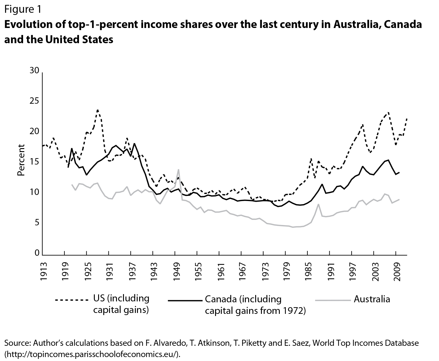
Figure 1 shows that the overall trend in the top 1 percent share has followed a similar U-shaped pattern in Canada and the United States (and in the UK and Australia) over the past century: very high in the 1920s and 1930s, declining in the 1940s and early 1950s, stabilizing in the 1960s and 1970s and increasing strongly since the early 1980s (see also Alvaredo et al. 2012; Heisz, figure 6, in this volume, and Atkinson and Piketty 2007).
In Australia — unlike in Canada and the United States, where the median real wage and the average income of the bottom 90 percent have stagnated — middle-class incomes have risen appreciably in recent years. Greenville, Pobke and Rogers (2013) argue that, since 1988, the longest resource boom in -Australian economic history has produced significant increases in employment, hours of work and the hourly real wage for the middle quintiles of the income distribution. Relying on survey data from the Household Expenditure Survey, they note that “rising inequality in Australia is also driven by the 99 percent, not just the 1 percent” (2013, 9).
Nevertheless, in Canada, the United States and Australia, the further up the income pyramid one goes, the faster the rate of increase of income. Figure 2 compares the long-term compound annual growth rate of real taxable income for various segments of the income distribution.11 Australia stands out for the positive (+1.13) growth rate of average real taxable annual income among the bottom 90 percent of tax units. However, all three countries share the pattern of unequal growth, with an accelerating rate of increase in real incomes at the top. Since the gulf between income groups will continue to widen as long as incomes at the top end grow faster than the incomes of everyone else, all three countries face the problem of unbalanced growth — income inequality will continue to increase until either bottom-end incomes grow much faster or top-end incomes grow much slower.
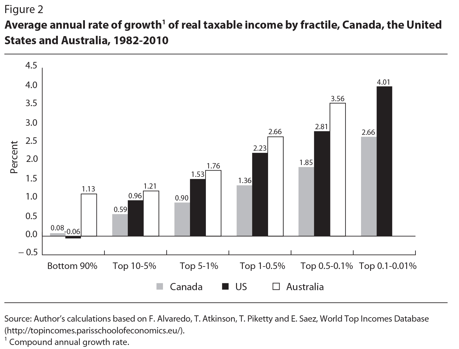
The income share of the top 1 percent is the ratio of the total income of the top 1 percent to the total income of all persons (the bottom 99 percent plus the top 1 percent). A ratio changes over time if the rate of growth of the -numerator differs from the growth rate of the denominator. In Canada and the United States, stagnant average real incomes of the bottom 90 percent contrast with the strong growth of incomes at the top, but middle-class income growth is not, by itself, necessarily enough to prevent rising inequality. The bottom 90 percent of -Australians did get some increase in average real income: 1.13 percent growth per year compounds, over 28 years, to a 32 percent real increase, which is much preferable to the cumulative real gains of the bottom 90 percent of -Canadians (2.1 percent) and Americans (– 1.5 percent). Nevertheless, the differential in income growth rates across income groups still produced a similar trend of rising income shares at the very top.
Although the income share of the top 1 percent declined from the late 1930s to the mid-1970s in all three countries (see Heisz, in this volume, figure 6, for Canada and the United States), this was not due to an actual decline in the real incomes of the top 1 percent. Rather, the drop in their income share was driven by the more rapid growth of real incomes of the other 99 percent of the income distribution. The income levels of the top 1 percent in real, local dollar terms did not decline prior to 1980; they just grew slowly (Osberg 2014, 16). Since the early 1980s, however, the incomes of the top 1 percent have grown dramatically — an upward trend to which there is no obvious upper bound. As figure 2 illustrates, income growth rates have been even larger the further up the income distribution one cares to look. Lemieux and Riddell (in this volume, 112) note that, “because there are not as many people (relative to population) with extremely high incomes in Canada as there are in the United States, fractile-based comparisons of incomes at the top refer to people with substantially different levels of incomes.” The key point, however, is that increasing shares of taxable income held by the top 1 percent of the distribution since the early 1980s have been driven by imbalances in growth rates across the income distribution.
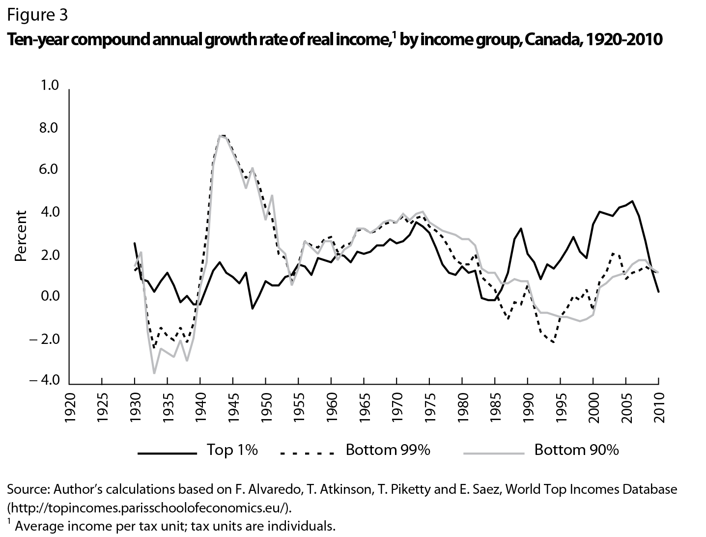
To show the changes over time in relative income growth rates underlying the changes in income shares, figure 3 plots the 10-year compound rate of real growth of average income of the top 1 percent, bottom 90 percent and bottom 99 percent in Canada since the 1920s, while figure 4 does the same for the United States. Figure 3 shows a 30-year period in Canada (from the early 1950s to the early 1980s) of rough equality in income growth rates between the top and the bottom ends of the distribution, sandwiched between long periods of unbalanced growth. The 1953-85 period of balanced growth meant stability in the distribution of income. However, from 1939 to 1952 the much more rapid growth of incomes at the lower end produced greater equality of income, while over the past 30 years, the more rapid growth of incomes at the top has produced greater inequality.
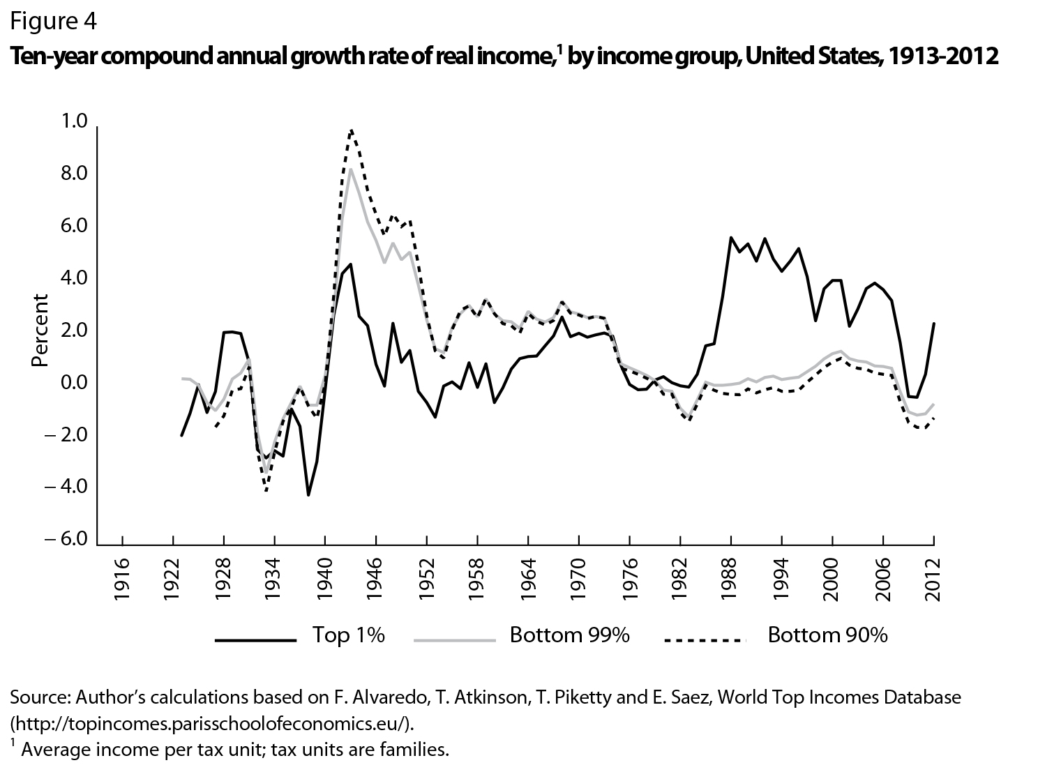
In the United States, income growth rates for the three income groups were nearly identical from 1967 to 1982 and quite similar from 1952 to 1967 — in total, a roughly 30-year period. However, figure 4 also shows dramatic differences in income growth rates in the 1940s and again since 1980. As in Canada, the income of those at the bottom end grew much more strongly than the income of those at the top end in the 1940s, and US income inequality lessened dramatically, but the past 30 years have been dominated by the opposite dynamic.12
The rapid growth of real incomes of the bottom 90 percent in Canada and the United States after 1940 started from a situation in which
In addition, the initially low share of women in the paid labour force meant that rising female employment could have a big impact on disposable household income. Finally, in the political economy of social policy, the “hard left” political option had a “threat effect” on political elites, who agreed to progressive taxation and the expansion of transfer programs that recycled top-end incomes.
Although wartime mobilization and controls were “once-only” events, the structural changes of economic development — urbanization, rising female labour force participation, widespread secondary and postsecondary education — had a large effect on family incomes. This effect was spread over a number of years and showed up as an increase in the growth rate of average income in the postwar era. Part of the reason the bottom quintiles of the income distribution in Canada and the United States have experienced smaller increases in income over the past 30 years than in earlier decades is that these structural changes were completed by 1980. Overall, however, balanced growth is not the norm. The 30-year period between 1952 and 1982 appears to have been a happy accident of history during which income growth rates at the top and the bottom were roughly equal. Balanced growth then made it plausible to ignore changes in the income distribution and to emphasize the steady-state -properties of economic systems inhabited by “representative agents.” But this period was a historical anomaly. Since the early 1980s, unbalanced income growth at the top has become the “new normal.”
A differential of 2 or 3 percentage points in the annual income growth rates of different income groups does not sound like much. Indeed, if the differential were short-lived, it would not amount to much. But this reality has been with us for three decades now. What will the future look like if this trend continues? As table 1 shows, the result will be ever-larger absolute differences in income and an ever-increasing ratio of the top 1 percent’s income to income in the rest of the income distribution.
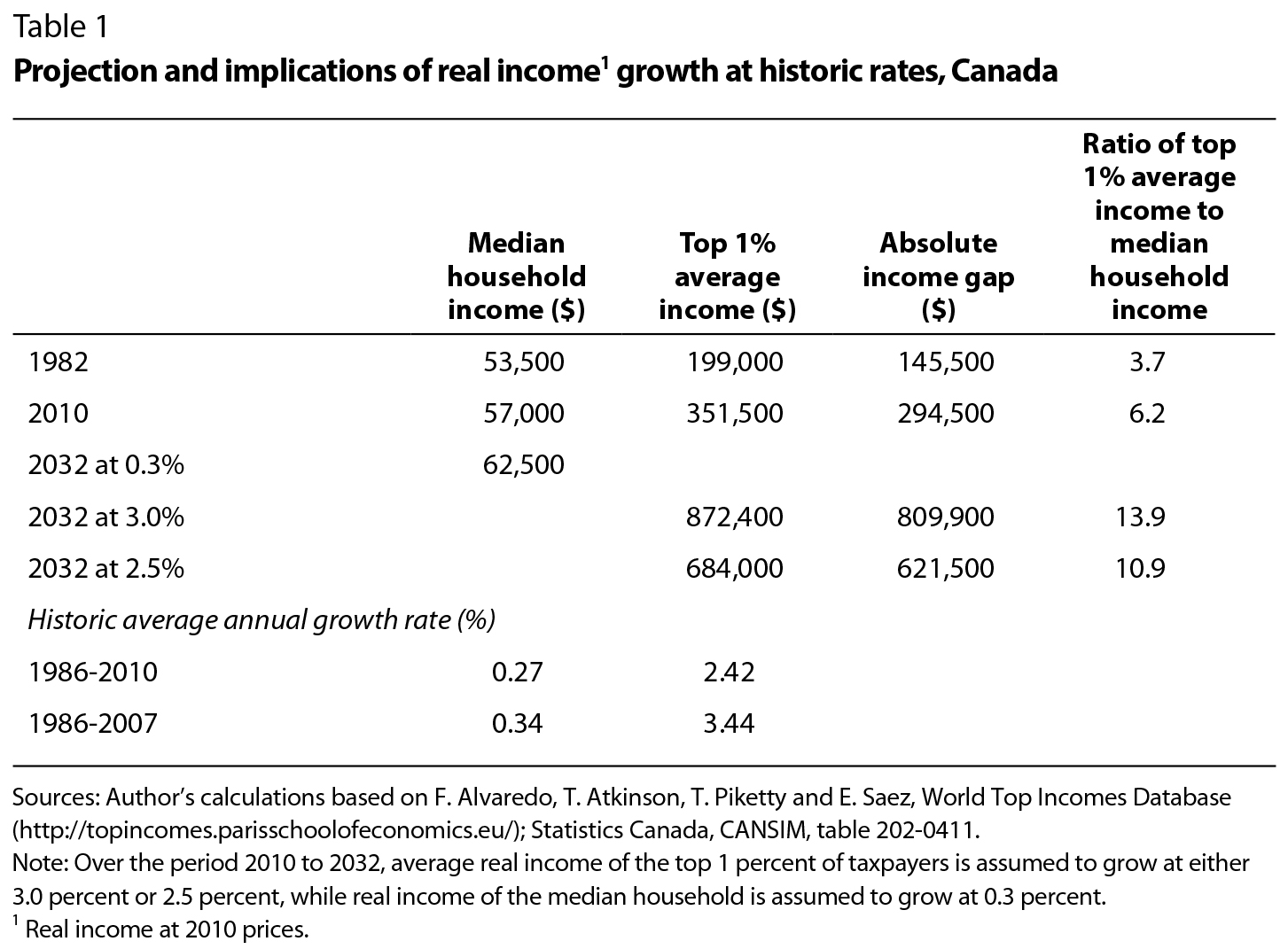
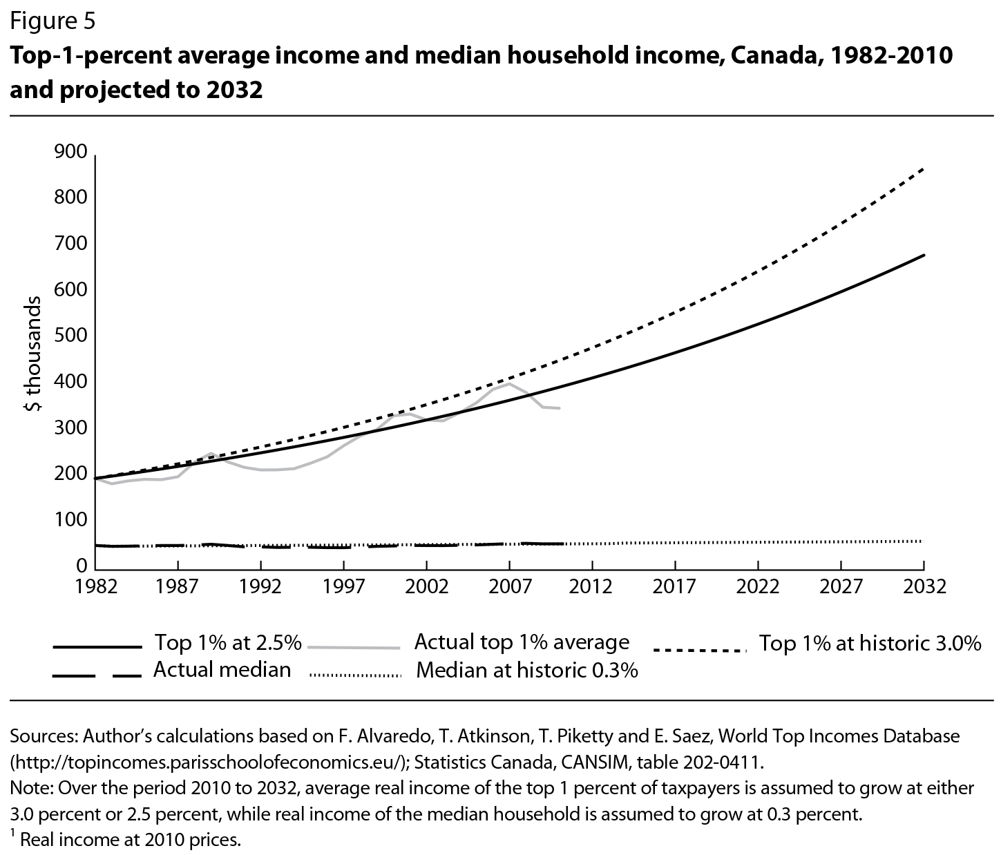
Figure 5 plots the average real income (excluding capital gains) of the top 1 percent and real median household income in Canada from 1982 to 2010, and presents two projections out to 2032. The first projection assumes a compound annual income growth rate of 3.0 percent for the top 1 percent, and the second assumes a slightly lower rate of 2.5 percent. The growth rate of median household income is assumed to be 0.3 percent.
In a recent study (Osberg 2014), I present similar calculations for the United States. Because the average of the top 1 percent of taxpayers in the United States is compounding at a faster rate (3.5 percent) on a larger base ($1,022,000 in 2012), emerging income gaps in that country are much bigger than in Canada. Specifically, the annual gap between average income in the top 1 percent and median income in the United States can be expected to swell from $970,700 in 2012 to $1,977,000 in 2032, while the income ratio, which was 8:1 in 1982 and 20:1 in 2012, can be expected to swell to 38:1 in 2032. In Canada, the income gap between the top 1 percent and the median household is less than that in the United States and is growing more slowly — but in both countries, it is historically large and growing steadily larger. What plausible market mechanism could be expected to change the underlying income growth rates that otherwise will produce this growing income gap?
Increasing income inequality over time and more rapid income growth at the top are just two different ways of describing the same reality. Stabilizing the income distribution requires income growth rates to be the same everywhere — either an acceleration of the income growth rate of the bottom 99 percent or a decline in the income growth rate of the top 1 percent could accomplish this result. Is enough of either likely to happen as a result of spontaneous “equilibrating” market forces?
If the issue was the division of national income between labour and capital, there might be grounds for optimism. For many years, this was seen as the “primary problem” of political economy (see Ricardo 1831). Neoclassical economists argued that, since the accumulation of capital by firms means a rising capital–to-labour ratio, the consequent diminishing marginal productivity of capital and rising marginal product of labour would produce rising wages and a decline in the rental rate of capital — which implies a tendency to restore stability in factor income shares. Indeed, generations of neoclassical economists have been brought up on the hypothesis that the Cobb-Douglas production function — which was devised precisely to explain the constancy of factor shares in the distribution of income despite an increasing capital-to-labour ratio — is a reasonable approximation of the actual technical relations of production.
If an accounting of “capital’s share” of national income included income derived from control over capital, as well as formal ownership of capital, most compensation of senior executives would be part of capital’s share, and the factor origins of the income of the top 1 percent would look different. In an earlier study (Osberg 2008), I noted that, in Canada, “labour’s share” of aggregate output has been declining since 1982; Lemieux and Riddell (in this volume) show how that trend is accentuated if the labour income of the top 1 percent is excluded. As well, the current labour earnings of the top 1 percent eventually will produce capital income from savings and inheritances. As Piketty (2014) emphasizes, when the interest rate exceeds the growth rate, there is a long-run tendency for capital’s share to increase. He also notes that the tendency for an increasing long-run concentration of capital ownership is particularly strong when the real rate of return is higher for large wealth holders — which means inheritance becomes an increasingly important aspect of ever-growing inequality.
Nevertheless, in Canada the main event so far has been the annual increase in top-end labour income. As Lemieux and Riddell (in this volume, 118-119) note, “Labour earnings…have been by far the largest source of income of individuals in the top 1 percent” (see also Alvaredo et al. 2013; Leigh 2013; Veall 2012). Hence, because the increasing inequality of the past 30 years has been the inescapable result of the difference between the long-term rate of income growth of the top 1 percent and that of everyone else, the question is whether, in the medium term, any automatic mechanism of self-adjustment in the labour market could restore balanced growth in labour incomes and thereby stabilize market income inequality.
One possible (if not very realistic) model of the labour market that does have an automatic self-adjustment mechanism is the hypothesis that top-end incomes have been growing rapidly solely because of increased work effort. Hours of work hit a physiological maximum somewhat before 6,000 per year — that is, 16 × 365 = 5,840.13 Work intensity per hour is less easy to measure, but it is implausible to think it can increase without limit. Because the top 1 percent cannot increase their labour supply forever, increases in income that are due to increases in effort eventually have to stop.
A labour supply explanation for the rapid income growth at the top end appeals to the possibility that greater “incentives” — in the form of significant cuts in top marginal tax rates since the 1980s — might have motivated an increase in the level of effort exerted by corporate executives and other highly paid professionals.14 This perspective fails, however, to explain the timing of income increases (see Milligan and Smart 2014; Veall 2012). It also cannot explain the much greater proportionate increases in income that have occurred the further one goes up the income distribution. As figure 2 shows, the incomes of the bottom half of the top 1 percent grew much less rapidly than the incomes of the next four-tenths of the top 1 percent or the incomes of the top one-tenth of the top 1 percent. As a result, in the United States by 2012, the top 1 percent had increased their average income (excluding capital gains) to 288 percent of the 1982 level, the top 0.5 percent to 331 percent of the 1982 level, and the top 0.1 percent to 451 percent of the 1982 level. If these increases were due solely to increased work effort, this would imply that the top 1 percent were working only about a third (34.7 percent) as hard in 1982 as in 2012, the top 0.5 percent were working just 30 percent as hard in 1982, and the top 0.1 percent were slackers 30 years ago, working only 22.2 percent as hard as in 2012. Is it likely that the elite in 1982 were really that much lazier than the elite 30 years later?
It is much more plausible to think that the people at the top of occupational and organizational hierarchies have always worked hard to succeed, that such social positions are rationed and that the top end of the labour market is effectively segmented from the general labour market. A more realistic model of the labour market is one in which pay at the top of the corporate heap depends on firm size, and for oligopolistic and monopolistically competitive firms, size depends on the scale of the market (Gabaix and Landier 2008). Since 1980, many firms in -Canada, the United States and Australia that previously operated on a national scale have expanded into global markets as trade barriers and transportation costs have fallen and managerial innovations, telecommunications and information systems have made effective management of large, dispersed organizations more feasible. As the scale of these firms’ global operations and global profits grows, their top management team takes a share — and the rents to their hierarchical positions increase with their rank in the hierarchy and with market size (which is growing at the global growth rate).15
In entertainment and sports, audience size has similarly grown, at least for those at the top who can now reach global audiences. The outsized returns obtained at the top end of financial services also rely on the scale of financial markets and on individuals’ placement in the hierarchy of market differentiation — again, rents to those in top hierarchical positions, whom Rosen (1981) describes as having “superstar” status, increase with the size of market supplied. Although individual markets and firms will grow at different rates, to a first approximation the average rate of growth of market size and, therefore, the average rate of income growth of “global” players will be driven by the rate of growth of global markets, which has been significantly faster than domestic growth in Canada, the United States and Australia. Since one can expect continued rapid growth in China, India and elsewhere (including sub-Saharan Africa), there is every likelihood that the growth rate of global markets will continue to be considerably greater than that of domestic markets for many decades to come.
As global markets grow, and as the firms servicing those markets expand, top corporate pay packages grow. There is little real evidence, however, that the rate of income growth of those at the top is driven by a similar rate of growth of their executive skills — administrative hierarchies are a type of team production where accurate measurement of an individual’s true marginal product is rarely feasible. A more plausible model of the determination of top corporate pay is Lydall’s (1959, 1968) model of pay in hierarchies, which has long predicted that the steepness of the upper tail of the earnings distribution will depend on hierarchical rank, the span of control at each level of the hierarchy and wage norms. Norms of pay growth set at the very top of enterprises that service global markets attenuate somewhat within those hierarchies as they trickle down to less senior members of top corporate management.16 Norms, however, are central to the propagation of these wage trends because, first, they always matter hugely (see Doeringer and Piore 1971) and, second, at the top end of corporate and public sector hierarchies in rich countries, most needs for creature comforts have long since been satisfied. At this pay level, relative income is the remaining motivator of effort. Money income is the marker that indicates who is “winning” or “losing” in the race for success, but “winning” — or, at the very least, “keeping up” — is the main event.
The rate of growth of compensation of those at the top of global corporations therefore sets the benchmark for those at the top of the national private sector, which in time determines what their peers at the top of public sector hierarchies — such as university presidents and senior civil servants — come to expect as the “fair” rate of increase of normal remuneration. Hence, for “the globals and their peers,” who sit at or near the top of organizational and professional hierarchies, the rate of growth of globalized markets seems likely to assure continued increases in corporate scale and top pay. As hundreds of millions of newly -middle-class households around the world discover the pleasures of the globalized brands of consumer society, the rents available to oligopolistic firms grow and with them the salaries of their top management teams, with -trickle-down benefits for their peers in other sectors.
For present purposes, the bottom 99 percent of workers can be thought of as “locals” who are not linked to top-end internal labour markets and whose pay growth and employment prospects depend on the aggregate supply and demand for labour in their own national and local labour markets. If unions had been able to mobilize collective action effectively, they might have restrained the escalation of corporate norms of top pay (Western and Rosenfeld 2011) and bargained for a share of increasing global corporate rents — but private sector union membership has declined significantly in Canada and the United States over the past 30 years. Because global firms usually can site their production in many possible places around the world, international competition for new investment sets the growth of local labour productivity as an approximate upper bound to the rate of average income growth of local labour. Slack local labour markets, however, can mean that, as in Canada between 1980 and 2000, average real wage growth falls short of that upper bound. (The resources sector is a significant exception, since the immobility of resource extraction activity can enable workers in some specialized occupations and in “boom towns” to extract part of the resource rent, to an extent that depends on the speed of resource development and the level of unionization.)
In this perspective, the long-run constraint on the income growth rate of locals is the local rate of labour productivity growth, while the long-run income growth rate of “the globals and their peers” depends on the rate of growth of global markets, which is significantly higher. Although a full discussion of this perspective would require much more space, I outline it here to indicate that at least one coherent view of the world is consistent with a continuation of the long-run differential between the growth rate of market income for the top 1 percent and the growth rate for everyone else.
What is the alternative hypothesis? Why might the growth rate of the average income of the bottom 99 percent accelerate substantially enough to match the recent income growth rate of the top 1 percent? Why might the growth rate of the average income of the top 1 percent slow enough to match the income growth rate of the bottom 99 percent?
Could improving educational attainment significantly raise the long-run growth rate of the average income of the bottom 99 percent — that is, could education be, in the words of Leigh (2013), “the great equaliser”? There are many non-economic reasons to be in favour of improved education, not least of which is the impact of education on dimensions of life such as social capital and social cohesion (see Osberg 2003; Wolfe and Haveman 2001). As Fortin et al. (2012, 138) note, however, “Caution is required in thinking about education as an inequality reducing policy,” since under some circumstances it might not improve equality of pay.17 As well, even if improving educational attainment could reduce inequality of opportunity between the disadvantaged and the middle class and reduce wage differentials within the middle class (for example, the ratio between the average wage of those with a university education and those with high school),18 this would not necessarily accelerate the growth rate of the average income of the bottom 99 percent. As well, increased education has inherent upper bounds if educational quality is to retain its meaning, and since the gains from any increase in enrolment would be the gains of those who are now at the margin, diminishing marginal returns have to be expected. In Canada, for example, 56 percent of the 25 to 34 age cohort already have a tertiary education, which suggests that further expansion of tertiary education among that cohort likely will have to reach further into the lower tail of the IQ distribution.
Educational initiatives, moreover, inherently operate with long time lags. Even an all-powerful leader with a magic wand that could instantaneously and totally revolutionize primary and secondary education in 2015 would have to wait 12 years, until 2027, to see the full impact of this change on high school graduates. To improve educational attainment over current Canadian levels, some tertiary education would be needed, which would push the graduation date under a new education regime back to 2031 or later — by which time the income gaps depicted in figure 5 would already have fully emerged. Even then, aggregate impacts initially would be small, because the flow of new graduates entering the workforce each year is only about a 40th of the workforce, and the impact on average labour force skills is the differential between the skills of entering and retiring cohorts. Thus, it would be roughly another 20 years — that is, around 2051, or about 36 years after the change — before those new entrants made up the majority of the workforce.
Furthermore, Canada’s experience already offers a guide as to whether an expansion of education could really be expected to solve the inequality problem. For the 25-to-64 age group, Canada’s tertiary education attainment level (51 percent in 2010) substantially exceeds that of the United States (42 percent) or Australia (38 percent) — indeed, it is the highest among the OECD countries (OECD 2012). Canada’s investment in education has been a “good thing” for many reasons, but it has not accelerated the rate of income growth of the bottom 99 percent. Australia, despite coming last among the three countries in tertiary education attainment, is the only one that has seen appreciable real income growth for the bottom 90 percent in recent decades.
Macroeconomic policy can influence the level of income inequality when labour is underemployed. When there is slack in the labour market, lowering the unemployment rate increases incomes at the bottom end of the income distribution, both by increasing the hours of work of unemployed and underemployed workers and by putting upward pressure on the real hourly wage (see Peach, Rich and Cororaton 2011). Raising the long-run growth rate of the real income of the bottom 99 percent through macroeconomic stimulus, however, would require a continuous reduction in unemployment, which is not feasible. Thus, macroeconomic stimulus cannot be expected to change long-run income growth rates.
Which plausible model, then, predicts that the market mechanism, on its own and anytime soon, will either slow the growth rate of average income of the top 1 percent or increase the growth rate of average income of the bottom 99 percent to the extent that these growth rates are equalized? If there is no solid reason to expect growth rate convergence and if unbalanced income growth seems more likely to continue, what are some implications?
When the income share of the top 1 percent is small, changes in that share have general equilibrium effects and socio-political effects that also are relatively small. But as the income share of the top 1 percent increases, its impact also increases. Furthermore, the decline in marginal tax rates on top incomes, which has occurred in all three countries over the past 30 years, has meant that the top 1 percent have seen an even larger increase in their disposable post-tax income than in their pre-tax market income. Hence, in all three countries, the absolute size of the gaps in disposable income between the top 1 percent and everyone else has grown more rapidly than the gaps in market income. Unbalanced income growth — that is, increasing household disposable income inequality — has increasing effects over time as income gaps widen. Because increased income must be either consumed or saved, this raises two sets of questions: (1) What are the implications of increased savings by the top 1 percent, and (2) What are the effects of their increasing consumption?
Before attempting to answer these questions, one should add the important caveat that size matters. Since the United States is so much larger than Canada or Australia, and since global capital markets are linked, the savings of the top 1 percent in the United States are far more important to the stability of world financial markets than the savings of the top 1 percent in Canada or Australia. The real incomes of the US top 1 percent are already much higher than their Canadian or Australian counterparts (both absolutely and relative to median income), so the income gap is compounding in the United States at a higher rate on a higher base — and so becoming much bigger, much faster — than in the other two countries. Thus, at any point in time, the stresses implied by unbalanced growth will be greater in the United States than elsewhere.
The top 1 percent might choose to hold some of their savings directly, as real assets, but unless all of their savings always take this form, rising incomes at the top of the distribution imply an increasing flow of their savings into financial markets.19 But financial instruments are inherently both an asset for the holder and a liability to the issuer. Thus, for the increasingly affluent, as a group, to acquire ever more net financial assets, somebody else has to acquire ever more financial liabilities. Indeed, macroeconomic balance requires it: if aggregate expenditure is to equal aggregate income, whenever the increasingly affluent abstain from spending some of their increase in income, other agents must spend more than their income. By borrowing and spending, debtors — both households and governments20 — balance the real flows of the economy, simultaneously increasing their stock of debt.
If borrowing and spending are insufficient, at a given real rate of interest, to balance income and expenditure, the result is downward pressure on interest rates and aggregate output. Summers (2013, 2014) and others argue that the United States and European economies have a structural tendency to secular stagnation, while King and Low (2014) have documented the decline in the world real interest rate, particularly since 2000. When the general level of interest rates declines, investors seeking a target rate of return must assume increasing risk in their asset portfolios. In the actual historical context of the United States prior to 2007, the matching of willing borrowers and willing lenders was greatly -facilitated by higher housing prices (which allowed households to support consumption through refinancing their mortgages on favourable terms), financial innovation (which allowed banks to repackage these loans and sell them as financial assets) and a facilitative regulatory environment. This combination of factors -successfully maintained high aggregate demand and relatively low unemployment in the United States prior to 2007 even though continued stagnation of the incomes of poor and middle-income households meant that loans and leverage kept rising.
Kumhof and colleagues (Kumhof et al. 2012; Kumhof and Rancière 2010; Kumhof, Rancière and Winant 2013) note that both the Great Depression that began in 1929 and the Great Recession of 2007-08 were preceded by a sharp increase in income and wealth inequality and by a similarly sharp increase in the debt-to–income ratio among lower- and middle-income households. They argue that when that debt-to-income ratio began to be perceived as unsustainable, a financial crisis became inevitable, needing only a trigger. Using a general equilibrium model, they show that the key mechanism, reflected in the rapid growth in the size of the financial sector, is the recycling of part of the additional income gained by high-income households back to the rest of the population by way of loans, thereby allowing the latter to sustain consumption levels temporarily and maintaining macroeconomic balance (Kumhof and Rancière 2010, 22).21 The slow growth of income of poor and middle-income households means, however, that their loan leverage keeps growing, and so does the probability of a major financial crisis, with severe implications for the real economy.22
This key idea — that ever-growing incomes at the top produce an ever–increasing flow of loanable funds, which eventually produces either a crisis in financial markets and a recession in the real economy or a period of secular stagnation — has a long history. In the nineteenth century, Marx argued strongly that cyclical instability was inherent in capitalism, while “underconsumptionists” such as Hobson ascribed the growth of British imperialism and overseas investment in the late 1800s to inadequate domestic absorption of the potential output of capitalism.23 Milanovic (2009) and others have also argued that the root cause of the 2008 financial meltdown was increasing income inequality.24
Before the 2007-08 recession, Leamer (2007, 1) argued that “housing starts and the change in housing starts together form the best forward-looking indicator of the cycle.” Periodic housing booms are fed by the cost and availability of credit and by self-reinforcing expectations of future increases in house prices. Owner-occupied housing is the main asset type held by middle-income households, and home mortgages enable financial leveraging to become a normal middle-class phenomenon, so middle-class net worth has become very sensitive to house price changes25 and interest rates, both of which are quite variable. As households become more indebted, their probability of default increases and financial assets become increasingly fragile.
The debt-stability equation has been most often used in the context of public sector finances, but its logic is equally applicable to households and the private sector. It starts from the accounting identity that the face value of the stock of an agent’s debt at a point in time is equal to the previous period’s debt plus interest accruing minus any “primary balance” surplus of income over current spending that is used to pay back the debt. The burden of debt depends on its size relative to income. For public finances, the ratio of debt to gross domestic product (GDP) is the crucial economic statistic, while each household confronts its personal ratio of household debt to household income.26 When income grows faster than debt, the debt-to-income ratio declines; if debt and income grow at the same rate, the ratio of the two is constant. In either event, debt is on a sustainable path. If the debt-to-income ratio is increasing over time, however, an ever-larger fraction of expenditure must go to servicing the debt rather than to financing current spending, a process that is eventually unsustainable.27
These debt dynamics can be summarized in the following equation:
∆(D/Y)t = (rt – gt)*(Dt-1/Yt) – (PBt/Yt), (1)
where Dt = debt in period t, rt = the average rate of interest in period t, PBt = the primary balance in period t, Yt = income, gt = the growth rate of income and ∆(D/Y)t = the change in the debt-to-income ratio. The first term makes clear how much debt stability depends on the interaction between the overhang of debt from the past (Dt-1/Yt) and the differential between the interest rate and the growth rate (rt – gt). Whenever the interest rate exceeds the income growth rate (that is, when rt – gt > 0), past debt is compounding faster than income is growing — and when the stock of past debt starts to feed on itself in this way, the primary balance surplus of current receipts over current spending must be continual and increasing just to stabilize the debt-to-income ratio.
Furthermore, the dilemma for the real-world public sector is that countercyclical spending by governments, in response to the collapse of real output and employment occasioned by the financial crisis of 2008, added to the stock of outstanding government debt. But equation (1) implies that, when the growth rate is less than the interest rate and the debt-to-GDP ratio is large, big increases in revenues and/or cuts to expenditures are necessary to offset the compounding of past debt. The macroeconomic implication of this additional fiscal drag is reduced GDP growth, thereby worsening the debt-to-GDP ratio. Because international bond traders are highly aware of the mathematics of debt stability, their changing anxieties can produce sudden surges in the interest cost of refinancing the maturing debt from past periods.
In the United States, the ratio of federal debt to GDP increased from 34.6 percent in 2001 to 86.5 percent in 2012 and continues to rise; in the eurozone, the government debt-to-GDP ratio reached 106.9 percent in 2013. As long as interest rates on new debt are kept near zero, the cost of refinancing this debt will be minimized, but equation (1) implies that any eventual increase in interest rates will have huge implications for budget balances. Hence, the question everywhere is, “How long can ultra-low interest rates continue?”
The ripples of unbalanced growth and instability thus lead to unpleasant choices. Fiscal austerity might stabilize public budget balances, at the cost of depressed growth, rising unemployment and social unrest. A low-interest-rate mone-tary policy could maintain consumer demand and prop up the housing sector, but the longer it continues the greater will be the indebtedness of households and the vulnerability of housing prices and household finances to interest-rate increases. If and when inflationary pressures are combated, monetary authorities will have to use the policy lever of an increase in interest rates (rt) to reduce the rate of growth of aggregate demand and household income (gt), thus widening the differential (rt – gt) at both ends. Equation (1) tells us that, when the debt-to–income ratio is large, as it now is for both governments and households, a widening differential between the interest rate and the growth rate implies that expenditure cuts will also have to be large to create continuing current surpluses big enough to prevent the debt-to-income ratio from compounding unsustainably.28
In the public sector, large expenditure cuts to “entitlement” programs could help balance annual budgets. Cuts to the “social wage,” however, would accentuate the long-term relative impoverishment of the middle and lower quintiles of the income distribution, further slow the growth of their real incomes and make household “deleveraging” more difficult. If all sectors attempted to deleverage simultaneously, a recession would have to be expected, in which case even slower real income growth at the bottom of the income distribution would accentuate rising household income inequality and reinforce the imbalance of saving and consumption that initially helped create financial instability.
To summarize, from a macroeconomic perspective, ever-increasing income inequality cannot be a steady state. When income growth rates are unbalanced, one instability leads to another. Pressures intensify over time as the increasing income share of the top 1 percent implies their savings flows become an increasing fraction of GDP. Because financial and real flows are interdependent, and because flows accumulate to become stocks, an imbalance in income growth rates produces changing flows of consumption and savings, which compound into a rising stock of financial wealth at the top and a greater stock of indebtedness elsewhere. Increasing financial fragility then increases the probability of a financial crisis, with big impacts on real economic activity. When governments respond with deficit spending, this accumulates as public debt, which itself becomes increasingly fragile whenever interest rates exceed the growth rate. But if interest rates are kept low to stimulate consumer demand, households acquire levels of private debt that they might be able to finance only if ultra-low nominal interest rates continue indefinitely.
Although the increasing savings of the top 1 percent might be largely invisible to the other 99 percent, their increasing consumption cannot be completely hidden. Indeed, as Veblen (1912) noted over a century ago, conspicuous consumption is a large part of why some people want great wealth in the first place. But others often resent “if you’ve got it, flaunt it” lifestyles. So the socio-political question is, “Can the increasing consumption gap driven by the growing income gap shown in table 1 and figure 5 be consistent with long-run social stability?”
A high but stable level of inequality (as observed in, for example, medieval Europe or Mogul India; see Milanovic, Lindert and Williamson 2011) can enable the elite to develop strong norms of gracious living. If income differentials remain roughly constant, the seeming permanence of an income gap can over time habituate the masses to traditional differentials and acquiescence in their own place in life (a process that historically was reinforced strongly by organized religion). Films and television dramas such as Downton Abbey, which celebrate both the ostentatious consumption of the nobility and the faithful deference of their loyal retainers, portray the sociological reality that highly unequal ways of life can become part of definitions of self-identity. Viewed from a macroeconomic perspective, the extravagant consumption of the gentry serves to recycle income — and the fact that it was done in much the same way, year after year, meant that, for both servants and served, a given level of great inequality could become viewed as the “natural order of things.”29
The British servile tradition was built up over centuries, however, and current reality in Canada, the United States and Australia is quite unlike such earlier periods of high but stable inequality. Unbalanced growth and rapidly increasing real income differentials now create the problem (at the top) of finding, every year, new ways to consume — that is, the elite must be increasingly extravagant over time if their increasing income is to be recycled in consumption. With the continuation of the income growth rates of recent decades into the future, the absolute size of annual increments to income at the top will continue to swell — indeed, a 3.0 percent income growth rate implies that, in 24 years, these income increments will be more than twice as large as they are currently. Hence, ever-growing ostentation has to be expected.
To some extent, the top 1 percent already consume their income in a separate world of gated resorts and exclusive neighbourhoods that most of the other 99 -percent never see. As the absolute size of income differences increases, it will become increasingly difficult for the top 1 percent to socialize across income classes, and their social contacts will converge increasingly on their peers. As well, over time, the increasing magnitude of consumer expenditures by the top 1 percent will sustain an ever-growing infrastructure of inequality (in the form of high-end shops, five-star resorts, luxury car dealerships and so on) as ever more entrepreneurial energy is devoted to the design, production and marketing of separate spheres of exclusivity. Hence, as their incomes diverge increasingly from the median, the top 1 percent will gradually become more disconnected from the lived reality of the 99 percent. But what is the cost of all this to the 99 percent? Should they just try to think of the top 1 percent as self-exiling themselves to reservations where they can be ignored (and perhaps somewhat taxed)? What are the negative effects — the “externalities” — to the 99 percent of the continuing growth of top-1-percent income and consumption?
The process of increasing indebtedness of the middle class will be more rapid if consumption norms are relative. Bertrand and Morse (2013) show that greater inequality at the local level increases consumption by the middle class by shifting their consumption aspirations upward. When, for example, the top 1 percent build larger houses, they shift the frame of reference that defines what others slightly below them on the income scale consider an acceptable or desirable house, which in turn shifts the frame of reference for those just below them and so on all the way down the income distribution. As consumption norms shift upward, individuals experience a loss of utility from the consumption of goods that only recently were “good enough.” The social visibility and positional nature of housing make it a good example of comparative consumption, and (as already noted) it is also a key sector for business cycle dynamics. If norms of consumption are relative, there is both a direct utility effect on the 99 percent and an increase in business cycle risks.
Medieval Europe and Mogul India may have had extreme inequality (see -Milanovic, Lindert and Williamson 2011), which lasted for centuries, but neither had an advertising industry. In the twenty-first century, one can expect advertising to increase market envy and stoke discontent. As income at the top grows more rapidly than income elsewhere, luxury goods will grow as a fraction of total consumer spending. In the United States, the income share (including capital gains) of the top 1 percent was 10.8 percent in 1982, had risen to 22.5 percent by 2012 and, if historic income growth rates continue, will rise to over 30 percent by 2025. The large and increasing relative size of the top-end market is a powerful incentive for an ever-increasing volume of aspirational advertising.
Because the necessities of life must be purchased even if they are not advertised at all, any advertising of necessities focuses heavily on conveying price information. But since luxury goods are inherently discretionary expenditures, and because the top 1 percent already have all normal creature comforts, they have to be convinced somehow to purchase such goods. Luxury goods are thus necessarily advertising-intensive items that appeal to ideas of exclusivity and status to motivate sales.
Status goods, such as watches costing thousands of dollars, can command a premium price only if they are widely known to be status goods — there is no point paying thousands for a fancy watch if no one else recognizes it as “special.” Hence, advertisers have to market luxury goods, like expensive watches, both to those who can afford to buy them and to those who can’t, in order for those who do buy to know that everyone else knows that these are very expensive, very exclusive items. And although some status goods can acquire their cachet by tradition and word of mouth, the expanding pool of disposable income among the affluent creates ever-greater incentives to create new status goods using advertising. In such marketing campaigns, desire is created by the message that “everybody wants this, but only special people have it” — that is, by inspiring envy among those who do not possess the good, so that those who do buy it can have status and deference. Because the market value of luxury brands will depreciate without continued advertising to reinforce their message of exclusivity, privilege and wealth, mass media become increasingly saturated with their messaging.
Continually increasing income gaps between those at the top end and everyone else are therefore likely to imply a continuing shift in production toward advertising-intensive luxury goods and increasing incentives to produce ever more advertising messaging that tells the 99 percent what only the top 1 percent can buy and the 99.9 percent what only the top 0.1 percent can afford. As income differentials grow, the benchmarks of luxury will move ever further from the consumption norms of the median household, thereby ensuring that the less affluent are told increasingly frequently about the pleasures of goods they cannot afford.
Increasing income inequality in a market economy therefore creates greater incentives for advertising expenditures that cause envy. For the 99 percent, an externality of rising top-1-percent incomes is the increasing volume and ever-changing messaging associated with this pervasive bombardment of advertising. The aim of aspirational advertising is to create product awareness in the broader audience to motivate purchase of the advertised commodity by the much smaller target clientele. As such advertising increases, and is increasingly tilted toward emphasizing the importance and desirability of goods that most people cannot afford, the likely outcome is greater discontent and less human happiness among the 99 percent.
The bottom 99 percent might wish to ignore the top 1 percent, but the top 1 percent do not want to be ignored, either politically or socially. Increasing income inequality gives the top 1 percent ever more resources to intervene in the political process and to ensure that their opinions matter. In the United States, there is clear evidence (see, for example, Page, Bartels and Seawright 2013) that
As Stiglitz (2012) and many others have emphasized, the increasingly separate world of the top 1 percent and their growing influence over the political process diminish the relative influence of the rest of society to a degree that will increase over time if election spending is unconstrained (as in the United States and Australia). In Canada, one can expect increasing pressure to erode constraints on campaign spending in elections and increasing spending between elections — by ostensibly “public interest” shell foundations — to influence the climate of opinion.
One can expect top-1-percent parents to try to pass on their advantages to their children — which means purchasing as much influence over the social mobility process as they can. Part of this can be explained as an “income effect” in the human capital model of intergenerational mobility (see, for example, Becker and Tomes 1979). As top incomes increase, affluent parents can be expected to spend part of their increased income on their children by purchasing greater enrichment expenditures and thereby further differentiating the school system.
The intergenerational human capital model, however, understates the consequences of increasing income inequality, because it omits any recognition of the scarcity and rationing of top positions. In that model, positional externalities are assumed to be zero, and all decisions are made by the household. For example, parents have to decide whether to pay Harvard’s tuition fees, but Harvard admits everyone whose parents are willing to pay enough. In the model, there is nothing competitive about life, since an improvement in the life chances of one family’s children has zero impact on the life chances of any other family’s children. If this were true, increased spending by the elite on their own children would not actually hurt anyone else. The reality, however, is that top positions are scarce — elite schools and universities deny admission to some applicants — which implies that an improved probability of success for others necessarily implies a poorer chance of success for oneself. Labour economists have long recognized that, when top slots are scarce, competition implies an aggregate overinvestment in individual efforts to get ahead, because no individual recognizes the externalities to others (in diminishing their probability of promotion) of their own increased striving (see Devaro 2006). As the gap between payoffs to positions widens, the incentives driving such overinvestment by individuals also increase.30
The dark side of intergenerational mobility is that those who are already at the top of the income distribution can only lose from future mobility — for the elite, the only mobility is downward. Hence, increasing income inequality and larger prizes for top jobs increase the “drop from the top.” Increasing income inequality means an increase in the potential costs of downward intergenerational economic mobility for the children of affluent families. The larger the income gap, the more affluent parents have to worry about their children’s potential competitors and the more important it becomes for rich parents to give their own children every possible advantage. Increasing inequality thus accentuates the elite’s reluctance to pay the taxes that could partially equalize opportunity by funding compensatory public expenditure on developing the human capital of poor children — because their own children have more to lose from better life chances for poor children. Over time, as the top end of the income distribution pulls further and further away from the median, the elite have an ever greater stake in preventing the downward mobility of their own children. As memories of a somewhat shared common childhood background in the public school system recede into stories about grandparents, it will become ever harder to maintain the myth of equality of opportunity. And the greater is the success of the top 1 percent in ensuring continued high socio–economic rank for their own children, the less are the life chances of children from poorer households for upward mobility. Hence, increasing inequality of opportunity is another externality of the increasing income gap.
When income ratios are roughly constant, the associated levels of political spending, enrichment expenditures on the children of the elite and advertising of luxury goods do not change much over time — and habituation might well dull any tendency toward discontent with inequality. But unbalanced growth implies increasingly large absolute income differences between income classes, increasingly large expenditures by the elite to influence the political process and to secure the advantages of their children and ever-increasing advertising reminding everyone of the desirability and exclusivity of the luxury goods that most people cannot -remotely afford. Is it likely that all such increases could continue indefinitely?
Cross-country comparisons indicate (unsurprisingly) that more inequality of income is a good predictor of more inequality of opportunity and less intergenerational social mobility. Such comparisons depend, however, on stability of the level of income inequality, which in turn requires equal rates of income growth at all percentiles of the income distribution. If income growth is unbalanced — specifically, if the rate of growth of real income of the top 1 percent is significantly higher than that of everyone else — then more inequality over time is inescapable. In Canada, the United States and, to a somewhat lesser degree, Australia, such unbalanced growth has been the new normal for the past 30 years. If these differentials in income growth rates continue, they will compound to successively larger gaps between the top 1 percent and everyone else.
Equalizing the growth rate of market income across the income distribution requires either slowing the growth rate of income at the top or substantially accelerating the income growth rate at the bottom (or some combination of both). There is, however, no plausible mechanism by which market forces can be expected to produce enough of either trend anytime soon. Since a continuation of unequal growth rates implies ever-growing market income differentials and ever-growing savings and spending by the top 1 percent, unbalanced growth increases tendencies to both financial and real economic instability while heightening pressure on social stability, with serious implications as these trends interact.
Even if the growth rates of pre-tax market income remain unbalanced, more progressive income and wealth taxes, combined with redistributive transfers and -public spending, could in principle balance aggregate income and expenditure, equalize the growth rates of income and stabilize the distribution of household disposable income. Since savings and spending decisions are made with respect to post-tax, post-transfer income, instability issues would then become moot. Once the distribution of disposable income was stabilized, Canada then would face the problem of choosing which steady-state level of inequality would maximize social welfare.
However, decentralized market forces cannot be expected to equalize market income growth rates and stabilize income inequality spontaneously. When markets fail, as Samuelson (1958, 480) argued, “it is the task of political economy to point out where common rules in the sense of self-imposed fiats can attain higher positions of the social welfare function.” Although a full assessment of the probability that political economy will produce a desirable outcome is beyond the scope of this chapter, some historic precedents exist from the 1930s. In the United States, Franklin Roosevelt’s New Deal had multiple interlocking parts: countercyclical stimulus, regulatory reforms in financial and labour -markets, and more progressive taxation and social security. By restraining top-end income growth and assisting low-end growth, recycling fiscal flows and -regulating financial markets, these reforms stabilized US inequality dynamics for nearly 50 years — at a time when the overwhelming dominance and relative insulation from trade of the United States made “Stabilization in One Country” feasible. In Europe, the emergence of highly stable social democratic welfare states in the Nordic countries also dates from the 1930s.
In the multipolar globalized economy of today, can one expect individual nation-states to produce similar “common rules” that could stabilize income inequality? Rightly or not, policy-makers in smaller countries such as Canada fear the mobility of capital and highly paid labour should they attempt to impose higher marginal tax rates on top-end income.31 Offshore banking and sophisticated tax-avoidance strategies also limit the effective ability of smaller states to stabilize income inequality. If new coordination devices for the market economy are to be constructed, they might need to be international in scope, but international cooperation is difficult to arrange at the best of times.
What happens if such policy coordination does not occur and income growth rates continue to diverge? The social and economic instability of the 1920s and 1930s produced some positive examples of social choices, but it also produced Fascism in Italy and Spain and Nazism in Germany. Increasing income inequality is unsustainable in the long run, but it is not at all clear what economic and social instability might produce. In a dark scenario, instability could lead to increased social stress and potentially extremist social movements. If these were perceived as a threat to social order, and if they provoke an authoritarian response, an expansion of the surveillance state and a reduction of civil liberties also could well be part of “what’s so bad about increasing inequality.”
In a less pessimistic scenario, democratic political economy could rise to the challenge of increasing top-end marginal income tax rates to stabilize the after-tax income distribution — that is, equalize the growth rates of disposable income — then move to the socially preferred stable level of long-run inequality. Tax policy — specifically, substantial increases in top-end marginal income tax rates — is thus central to any realistic attempt to stop inequality increasing further. Left unchecked, the imbalances created by unbalanced growth will only get bigger over time, so increasing inequality is a challenge that Canadian governments eventually will have to face. But before Canadians can choose which stable level of inequality is desirable, they will first have to choose to stop inequality from increasing, year after year.
This chapter draws heavily on three linked papers with differing titles: “What’s So Bad about More Inequality?” (keynote address to the Academy of the Social Sciences in Australia — 2013 Annual Symposium, Canberra, November 12, 2013); “Canadian Inequality Then and Now: Can Increasing Inequality Be a Steady State?” (Galbraith Lecture, Progressive Economics Forum, Canadian Economics Association Annual Meetings, Vancouver, May 31, 2014); and “Can Increasing Inequality Be a Steady State?” Working Paper 56 (Paris: OECD, Statistics Directorate, June 18, 2014). Many revisions were made during a very pleasant sabbatical at the Statistics Directorate, OECD, whose hospitality is greatly appreciated. The comments of the editors and of Bruce Bradbury, Peter Burton, Mel Cross, Martine Durand, Talan Iscan, Brian MacLean, Marco Mira D’Ercole, Shelley Phipps, Peter Saunders (University of New South Wales), Andrew Sharpe, Paul Schreyer, Sy Spilerman, Ed Wolff and Armine Yalnizyan have greatly improved the chapter. In addition, the comments of participants in seminars at the OECD and at Columbia, Dalhousie and Griffith Universities, the Universities of New South Wales, Queensland and Lueneberg, and the National University of Ireland at Galway were very helpful. Errors remaining are entirely my own.
In economics, the neoclassical model of “steady-state” growth has argued that, with unchanging behavioural and structural characteristics, some ratios (such as per capita income or the capital/labour ratio) in principle can grow steadily for an indefinitely long time. The specific question asked in this chapter is whether the income share of the top 1 percent is a ratio that similarly can grow steadily indefinitely.
Aaron, H.J. 1978. Politics and the Professors. Washington, DC: Brookings Institution.
Alvaredo, F., A.B. Atkinson, T. Piketty, and E. Saez. 2013. “The Top 1 Percent in International and Historical Perspective.” Journal of Economic Perspectives 27 (3): 3-20. Accessed March 25, 2015. https://pubs.aeaweb.org/doi/pdfplus/10.1257/jep.27.3.3
Amdekar, S.D. 2012. “Inequality, Surplus Capital & Underconsumption: A Contemporary Analysis of J.A. Hobson’s Economic Theory of New Imperialism.” Working paper. University College, Durham University, Durham, UK.
Atkinson, A.B. 1970. “The Measurement of Inequality.” Journal of Economic Theory 2: 244-63.
Atkinson, A.B., and T. Piketty, eds. 2007. Top Incomes over the 20th Century: A Contrast between Continental European and
English-Speaking Countries. Oxford: Oxford University Press.
Atkinson, A.B., T. Piketty, and E. Saez. 2011. “Top Incomes in the Long Run of History.” Journal of Economic Literature 49 (1): 3-71.
Baker, D. 2006. The Conservative Nanny State: How the Wealthy Use the Government to Stay Rich and Get Richer. Washington, DC: Center for Economic and Policy Research. Accessed March 25, 2015. https://deanbaker.net:8080/images/stories/documents/
cnswebbook.pdf
Beaudry, P., and D.A. Green. 2003. “Wages and Employment in the United States and Germany: What Explains the Differences?” American Economic Review 93 (3): 573-602.
———. 2005. “Changes in US Wages 1976-2000: Ongoing Skill Bias or Major Technological Change?” Journal of Labor Economics 23 (3): 609-48.
Becker, G., and N. Tomes. 1979. “An Equilibrium Theory of the Distribution of Income and Intergenerational Mobility.” Journal of Political Economy 87 (6): 1153-89.
Bertrand, M., and A. Morse. 2013. “Trickle-Down Consumption.” NBER Working Paper 18883. Cambridge, MA: National Bureau of Economic Research.
Blau, F., and L.M. Kahn. 2009. “Inequality and Earnings Distribution.” In The Oxford Handbook of Economic Inequality, edited by W. Salverda, B. Nolan, and T. Smeeding. Oxford: Oxford University Press.
Bordo, M.D., and C.M. Meissner. 2012. “Does Inequality Lead to a Financial Crisis?” NBER Working Paper 17896. Cambridge, MA: National Bureau of Economic Research. Accessed March 25, 2015. https://www.nber.org/papers/w17896
Bowles, S., and H. Gintis. 1976. Schooling in Capitalist America: Educational Reform and the Contradictions of Economic Life. New York: Basic Books.
Bowlus, A.J., and J.-M. Robin. 2012. “An International Comparison of Lifetime Inequality: How Continental Europe Resembles North America.” Journal of the European Economic Association 10 (6): 1236-62.
Brunori, P.F., H.G. Ferreira, and V. Peragine. 2013. “Inequality of Opportunity, Income Inequality and Economic Mobility: Some International Comparisons.” World Bank Policy Research Working Paper 6304 and IZA Discussion Paper 7155. Bonn, Germany: Institute for the Study of Labor. Accessed March 25, 2015. https://ftp.iza.org/dp7155.pdf
Burkhauser, R., S. Feng, S.P. Jenkins, and J. Larrimore. 2009. “Recent Trends in Top Income Shares in the USA: Reconciling Estimates from March CPS and IRS Tax Return Data.” NBER Working Paper 15320. Cambridge, MA: National Bureau of Economic Research.
Burtless, G. 2009. “Demographic Transformation and Economic Inequality.” In The Oxford Handbook of Economic Inequality, edited by W. Salverda, B. Nolan, and T. Smeeding. Oxford: Oxford University Press.
Corak, M. 2004. “Generational Income Mobility in North America and Europe: An Introduction.” In Generational Income Mobility in North America and Europe, edited by M. Corak. Cambridge, UK: Cambridge University Press.
_____. 2013. “Income Inequality, Equality of Opportunity, and Intergenerational Mobility.” Journal of Economic Perspectives 27 (3): 79-102. Accessed March 25, 2015. https://pubs.aeaweb.org/doi/pdfplus/10.1257/jep.27.3.79
Cynamon, B.Z., and S.M. Fazzari. 2014. Inequality, the Great Recession, and Slow Recovery. Accessed March 25, 2015. https://dx.doi.org/10.2139/ssrn.2205524
Davies, J.B. 2009. “Wealth and Economic Inequality.” In The Oxford Handbook of Economic Inequality, edited by W. Salverda, B. Nolan, and T. Smeeding. Oxford: Oxford University Press.
Davies, J.B., S. Sandström, A. Shorrocks, and E.N. Wolff. 2010. “The Level and Distribution of Global Household Wealth.” Economic Journal 121 (March): 223-54. doi:10.1111/j.1468-0297.2010.02391.x
Devaro, J. 2006. “Strategic Promotion Tournaments and Worker Performance.” Strategic Management Journal 27 (8): 721-40.
Doeringer, P.B., and M.J. Piore. 1971. Internal Labor Markets and Manpower Analysis. Lexington, MA: D.C. Heath.
Dynan, K.E., J. Skinner, and S.P. Zelkes. 2004. “Do the Rich Save More?” Journal of Political Economy 112 (2): 397-442.
Fortin, N.M., D.A. Green, T. Lemieux, K. Milligan, and W.C. Riddell. 2012. “Canadian Inequality: Recent Developments and Policy Options.” Canadian Public Policy 38 (2): 121-45.
Frydman, C., and D. Jenter. 2010. “CEO Compensation.” NBER Working Paper 16585. Cambridge, MA: National Bureau of Economic Research. Accessed March 25, 2015. www.nber.org/papers/w16585
Gabaix, X., and A. Landier. 2008. “Why Has CEO Pay Increased So Much?” Quarterly Journal of Economics 123 (1): 49-100.
Gordon, R.J., and I. Dew-Becker. 2008. “Controversies about the Rise of American Inequality: A Survey.” NBER Working Paper 13982. Cambridge, MA: National Bureau of Economic Research.
Greenville, J., C. Pobke, and N. Rogers. 2013.
“Trends in the Distribution of Income in Australia.” Productivity Commission Staff Working Paper. Canberra: Government of Australia.
Hobson, J.A. 1900. The Economics of Distribution. New York: Macmillan.
_____. 1905. Imperialism: A Study. London: George Allen and Unwin.
Hou, F., and J. Myles. 2007. The Changing Role of Education in the Marriage Market: Assortative Marriage in Canada and the United States since the 1970s. Analytical Studies Branch Research Paper 299. Ottawa: Statistics Canada. Accessed March 25, 2015. https://www.statcan.gc.ca/pub/11f0019m/11f0019m2007299-eng.htm
Jenkins, S. 1991. “The Measurement of Income Inequality.” In Economic Inequality and Poverty: International Perspectives, edited by L. Osberg. Armonk, NY: M.E. Sharpe.
Joye, C. 2014. “House Prices ‘Flash Red’ as Debt to Income Ratio Hits Record High.” –Australian Financial Review, April 4.
Kaplan, S.N., and J. Rauh. 2013. “It’s the Market: The Broad-Based Rise in the Return to Top Talent.” Journal of Economic Perspectives 27 (3): 35-56.
King, M., and D. Low. 2014. “Measuring the ‘World’ Real Interest Rate.” NBER Working Paper 19887. Cambridge, MA: National Bureau of Economic Research. Accessed March 25, 2015. https://www.nber.org/papers/w19887
Kumhof, M., C. Lebarz, R. Rancière, A.W. Richter, and N.A. Throckmorton. 2012. “Income Inequality and Current Account Imbalances.” IMF Working Paper 12/8. Washington, DC: International Monetary Fund.
Kumhof, M., and R. Rancière. 2010. “Inequality, Leverage and Crises.” IMF Working Paper 10/268. Washington, DC: International Monetary Fund.
Kumhof, M., R. Rancière, and P. Winant. 2013. “Inequality, Leverage and Crises: The Case of Endogenous Default.” IMF Working Paper 13/249. Washington, DC: International Monetary Fund.
Leamer, E.E. 2007. “Housing IS the Business Cycle.” NBER Working Paper 13428. Cambridge, MA: National Bureau of Economic Research. Accessed March 25, 2015. https://www.nber.org/papers/w13428
Leigh, A. 2013. Battlers and Billionaires: The Story of Inequality in Australia. Collingwood, Australia: Black, Inc.
Leigh, A., C. Jencks, and T. Smeeding. 2009. “Health and Economic Inequality.” In The Oxford Handbook of Economic Inequality, edited by W. Salverda, B. Nolan, and T. Smeeding. Oxford: Oxford University Press.
Ljunggren, D. 2014. “Canada Household Debt-to-
Income Ratio Slips from Record High.” Reuters, March 14. Accessed March 26, 2015. https://www.reuters.com/article/2014/03/14/canada-economy-debt-idUSL2N0MA1I920140314
Lu, Y., R. Morissette, and T. Schirle. 2011. “The Growth of Family Earnings Inequality in Canada, 1980-2005.” Review of Income and Wealth 57 (1): 23-39.
Lydall, H.F. 1959. “The Distribution of Employment Incomes.” Econometrica 27 (1): 110-5.
_____. 1968. The Structure of Earnings. Oxford: Oxford University Press.
Mankiw, N.G. 2013. “Defending the One Percent.” Journal of Economic Perspectives 27 (3): 21-34.
Marshall, A. 1913. Principles of Economics. 8th ed. New York: Macmillan.
Marx, K. 1894. Capital. 3 vols. Repr., New York: International Publishers, 1967.
Milanovic, B. 2009. “Income Inequality and Speculative Investment by the Rich and Poor in America Led to the Financial Meltdown.” YaleGlobal Online, May 4. Accessed March 25, 2015. https://yaleglobal.yale.edu/content/two-views-global-crisis
Milanovic, B., P.H. Lindert, and J.G. Williamson. 2011. “Pre-industrial Inequality.” Economic Journal 121 (551): 255-72.
Milligan, K., and M. Smart. 2014. “Taxation and Top Incomes in Canada.” NBER Working Paper 20489. Cambridge, MA: National Bureau of Economic Research.
Morelli, S., T. Smeeding, and J. Thompson. 2014. “Post-1970 Trends in Within-Country Inequality and Poverty: Rich and Middle Income Countries.” CSEF Working Paper 356. Naples, Italy: Centre for Studies in Economics and Finance.
Murphy, B., S. Michaud, and M. Wolfson. 2008. “Income Trajectories of High Income Canadians 1982-2005.” Paper presented at the 30th General Conference of the International Association for Research in Income and Wealth, August 24-30, Portoroz, Slovenia. Accessed March 25, 2015. https://www.iariw.org/papers/2008/murphy2.pdf
Murphy, B., P. Roberts, and M. Wolfson. 2007. “High-Income Canadians.” Perspectives on Labour and Income 8 (9): 5-17. Accessed March 25, 2015. https://www.statcan.gc.ca/pub/75-001-x/75-001-x2007109-eng.pdf
New York State. 2014. Department of Taxation and Finance. “New York City Tax Rate Schedule.” Accessed March 26, 2015. https://www.tax.ny.gov/pdf/current_forms/it/nyc_tax_rate_schedule.pdf
OECD (see Organisation for Economic Co-operation and Development)
Organisation for Economic Co-operation and Development (OECD). 2011. Divided We Stand: Why Inequality Keeps Rising. Paris: OECD Publishing. doi:10.1787/9789264119536-en
_____. 2012. Education at a Glance 2012: OECD Indicators. Paris: OECD Publishing. doi:10.1787/19991487
Osberg, L. 1981. Economic Inequality in Canada. Toronto: Butterworths.
_____. 1984. Economic Inequality in the United States. Armonk, NY: M.E. Sharpe.
_____, ed. 2003. The Economic Implications of Social Cohesion. Toronto: University of Toronto Press, Toronto.
_____. 2008. A Quarter Century of Economic Inequality in Canada: 1981-2006. Toronto: Canadian Centre for Policy Alternatives. Accessed March 25, 2015. https://www.policyalternatives.ca/documents/National_Office_Pubs/2008/Quarter_Century_of_Inequality.pdf
_____. 2013. “Instability Implications of Increasing Inequality: Evidence from North America.” Economic Modelling 35: 918-30.
_____. 2014. “Can Increasing Inequality Be a Steady State?” OECD Statistics Working Paper 2014/01. Paris: OECD Publishing.
Osberg, L., and T. Smeeding. 2006. “‘Fair’ Inequality? Attitudes toward Pay Differentials: The United States in Comparative Perspective.” American Sociological Review 71: 450-73.
Page, B., I.L.M. Bartels, and J. Seawright. 2013. “Democracy and the Policy Preferences of Wealthy Americans.” Perspectives on Politics: 11 (1): 51-73.
Peach, R., R. Rich, and A. Cororaton. 2011. “How Does Slack Influence Inflation?” Current Issues in Economics and Finance 17 (3): 1-7.
Piketty, T. 2014. Capital in the Twenty-First Century. Cambridge, MA: Harvard University Press.
Piketty, T., E. Saez, and I. Stantcheva. 2014. “Optimal Taxation of Top Labor Incomes: A Tale of Three Elasticities.” American Economic Journal: Economic Policy 6 (1): 230-71.
Podoluk, J.R. 1968. Incomes of Canadians. Ottawa: Dominion Bureau of Statistics.
Pomerleau, K. 2014. “High-Income Taxpayers Could Face a Top Marginal Tax Rate over 50 This Tax Season.” Blog post, January 23. Accessed April 18, 2014. https://taxfoundation.org/blog/high-income-taxpayers-could-face-top-marginal-tax-rate-over-50-tax-season
Ricardo, D. 1831. The Principles of Political Economy and Taxation. Repr., New York: Dent, Everyman’s Library, 1969.
Rosen, S. 1981. “The Economics of Superstars.” American Economic Review 71 (5): 845-58.
Saez, E. 2013. Striking It Richer: The Evolution of Top Incomes in the United States (Updated with 2012 Preliminary Estimates). Accessed March 25, 2015. https://elsa.berkeley.edu/~saez/saez-UStopincomes-2012.pdf
Salverda, W., B. Nolan, and T. Smeeding, eds. 2009. The Oxford Handbook of Economic Inequality. Oxford: Oxford University Press.
Samuelson, P.A. 1958. “An Exact Consumption-Loan Model of Interest with or without the Social Contrivance of Money.” Journal of Political Economy 66 (6): 467-82.
Sawyer, M. 1976. “Income Distribution in OECD Countries.” OECD Economic Outlook, Occasional Studies. Paris: OECD Publishing.
Statistics Canada. 1998. Income Distribution by Size in Canada. Catalogue 13-207. Ottawa: Statistics Canada.
Stiglitz, J.E. 2012. The Price of Inequality: How Today’s Divided Society Endangers Our Future. New York: W.W. Norton.
Summers, L. 2013. “Why Stagnation Might Prove to Be the New Normal.” Financial Times, December 15.
_____. 2014. “Why Austerity Is Counterproductive in the New Economy.” Speech to the National Association for Business Economics, February 24, Arlington, VA. Accessed March 25, 2015. https://larrysummers.com/nabe-why-austerity-is-counterproductive-in-the-new-economy/
Tocqueville, A. de. 1831. Democracy in America, vol. 1. Repr., New York: Knopf, 1956.
Veall, M. 2012. “Top Income Shares in Canada: Recent Trends and Policy Implications.” Canadian Journal of Economics 45 (4): 1247-72.
Veblen, T. 1912. The Theory of the Leisure Class. Repr., New York: Mentor.
Western, B., and J. Rosenfeld. 2011. “Unions, Norms, and the Rise in U.S. Wage Inequality.” American Sociological Review 76: 513-37.
Wilkinson, R., and K. Pickett. 2010. The Spirit Level: Why Equality Is Better for Everyone. London: Penguin Books.
Wolfe, B., and R. Haveman. 2001. “Accounting for the Social and Non-Market Benefits of Education.” In The Contribution of Human and Social Capital to Sustained Economic Growth and Well Being: International Symposium Report, edited by J. Helliwell. Paris: Organisation for Economic Co-operation and Development; Ottawa: Human Resources Development Canada.
Wolff, E.N. 2011. The Transformation of the American Pension System. Kalamazoo, MI: W.E. Upjohn, Institute for Employment Research.
Wolfson, M.C., M. Veall, and N. Brooks. 2014. “Piercing the Veil — Private Corporations and the Incomes of the Affluent.” Working paper, School of Accounting and Finance, University of Waterloo. Accessed June 19, 2015. https://uwaterloo.ca/school-of-accounting-and-finance/sites/ca.school-of-accounting-and-finance/files/uploads/files/wolfson-brooks-veall_-_incomes_of_affluent.pdf
Yalnizyan, A. 2010. The Rise of Canada’s Richest 1%. Ottawa: Canadian Centre for Policy Alternatives.